Gradient Fields Forever

The gradient of a scalar field is one of the most powerful topics I’ve ever seen in mathematics. It is the, quite simply, the multidimensional generalization of the derivative. We can interpret it is a slope in more than one direction. For instance, in calculus, we deal with two-dimensional lines that go back and forth in the [latex]x[/latex]-plane and up and down in the [latex]y[/latex]-plane.

But imagine if, instead, we were standing on top of a hill. If it is a nice hill that is basically a bump in a field, we can stand on top and it goes down in every direction. There’s a slope in every direction and it is measured in two dimensions, how much it goes up and down over a distance back-and-forth and how much it goes up and down over a distance side-to-side. That’s a nifty little measure and with two distinct elements, is a vector that tells us how much the height of the hill changes and in what direction.

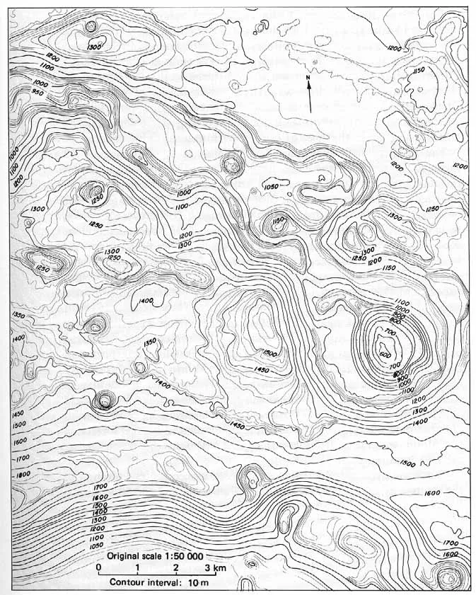
These vectors can be vastly simplified into contour lines. We see these contour lines in things like plat maps, engineering drawings, and similar. Here’s a neat example of Rima Prinz I on the Moon, produced by NASA as a part of the Apollo 8 mission.

There are other examples, too. If we take all of the individual gradients and place them in the points where they exist, you get a vector field. The vector field can show us in aggregate how everything holds together. Here’s another example of a vector field used to show the evolution of the May 24, 2017 tornado outbreak from the National Weather Service.

This is just a small part of the great things we can do with scalar fields and vector fields. It turns out, they are essential for modern machine learning techniques, but that’s a discussion for a different day.